22580: From GPT2 to Kimi3, Explained

By @waterloo_intern · 2026-07-27T15:22:08.000Z

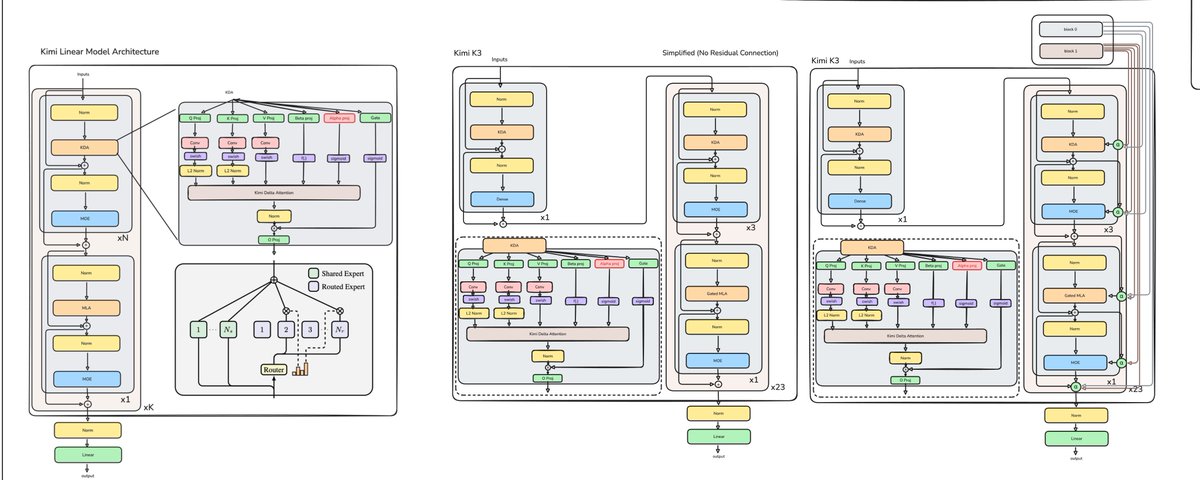
Twenty-two thousand five hundred and eighty. That’s how many GPT-2 (2019) models fit inside KimiK3 (2026). We scaled up by a factor of 22,580 in seven years. But is it just... scale?

In this worklog, I’ll walk through how we got here and how much, or how little, has actually changed since then. We’ll trace the major architectural developments leading to KimiK3.

GPT-2

GPT-2 is a decoder-only architecture:

tok_emb = self.transformer.wte(idx) # token embeddings of shape (b, t, n_embd)
pos_emb = self.transformer.wpe(pos) # position embeddings of shape (t, n_embd)
x = self.transformer.drop(tok_emb + pos_emb)
for block in self.transformer.h:
    x = block(x)
x = self.transformer.ln_f(x)
logits = self.lm_head(x)
return logits

The input receives token and positional embeddings:

Each transformer block, zoomed in, looks like this:

class Block(nn.Module):
    def __init__(self, config):
        super().__init__()
        self.ln_1 = LayerNorm(config.n_embd, bias=config.bias)
        self.attn = CausalSelfAttention(config)
        self.ln_2 = LayerNorm(config.n_embd, bias=config.bias)
        self.mlp = MLP(config)

    def forward(self, x):
        x = x + self.attn(self.ln_1(x))
        x = x + self.mlp(self.ln_2(x))
        return x

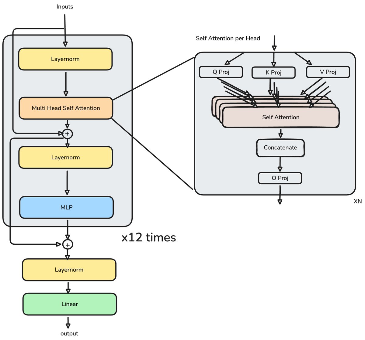
The attention process:

        B, T, C = x.size() # batch size, sequence length, embedding dimensionality (n_embd)

        # calculate query, key, values for all heads in batch and move head forward to be the batch dim
        q, k, v  = self.c_attn(x).split(self.n_embd, dim=2)
        k = k.view(B, T, self.n_head, C // self.n_head).transpose(1, 2) # (B, nh, T, hs)
        q = q.view(B, T, self.n_head, C // self.n_head).transpose(1, 2) # (B, nh, T, hs)
        v = v.view(B, T, self.n_head, C // self.n_head).transpose(1, 2) # (B, nh, T, hs)

        # manual implementation of attention
        att = (q @ k.transpose(-2, -1)) * (1.0 / math.sqrt(k.size(-1)))
        att = att.masked_fill(self.bias[:,:,:T,:T] == 0, float('-inf'))
        att = F.softmax(att, dim=-1)
        att = self.attn_dropout(att)
        y = att @ v # (B, nh, T, T) x (B, nh, T, hs) -> (B, nh, T, hs)
        y = y.transpose(1, 2).contiguous().view(B, T, C) # re-assemble all head outputs side by side

        # output projection
        y = self.resid_dropout(self.c_proj(y))
        return y

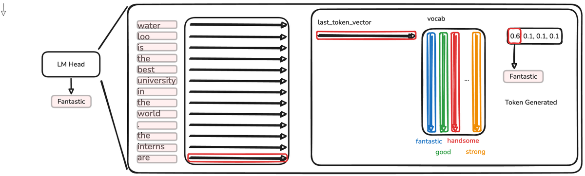
Once the final hidden-state matrix is produced, the language-model head maps it into vocabulary logits. During autoregressive decoding, only the logits at the final position are needed to select the next token.

This is an inefficiency of decoder-only generation: the model computes representations for every input position, but each decode step consumes only the final position’s logits. Without caching, much of that work would be repeated for the next token.

The KV cache comes from a straightforward observation: after appending the generated token to the input, the model would otherwise recompute projections for all previous tokens. Storing their key and value vectors avoids that redundant work.

That storage is the KV cache. It retains vectors for the previous N-1 tokens and can become large enough to create a memory-bandwidth bottleneck.

Overall, with about 50k possible tokens, 12 blocks, 12 heads, and an embedding dimension of 768, our baseline model is about 124M parameters.

vocab_size: int = 50304 # GPT-2 vocab_size of 50257, padded up to nearest multiple of 64 for efficiency
n_layer: int = 12
n_head: int = 12
n_embd: int = 768

At 2.8 trillion parameters, one KimiK3 model contains roughly as many parameters as 22,580 GPT-2 models.

tok_emb = self.transformer.wte(idx) # token embeddings of shape (b, t, n_embd)
pos_emb = self.transformer.wpe(pos) # position embeddings of shape (t, n_embd)
x = self.transformer.drop(tok_emb + pos_emb)
for block in self.transformer.h:
    x = block(x)
x = self.transformer.ln_f(x)
logits = self.lm_head(x)
return logits

class Block(nn.Module):
    def __init__(self, config):
        super().__init__()
        self.ln_1 = LayerNorm(config.n_embd, bias=config.bias)
        self.attn = CausalSelfAttention(config)
        self.ln_2 = LayerNorm(config.n_embd, bias=config.bias)
        self.mlp = MLP(config)

    def forward(self, x):
        x = x + self.attn(self.ln_1(x))
        x = x + self.mlp(self.ln_2(x))
        return x

        B, T, C = x.size() # batch size, sequence length, embedding dimensionality (n_embd)

        # calculate query, key, values for all heads in batch and move head forward to be the batch dim
        q, k, v  = self.c_attn(x).split(self.n_embd, dim=2)
        k = k.view(B, T, self.n_head, C // self.n_head).transpose(1, 2) # (B, nh, T, hs)
        q = q.view(B, T, self.n_head, C // self.n_head).transpose(1, 2) # (B, nh, T, hs)
        v = v.view(B, T, self.n_head, C // self.n_head).transpose(1, 2) # (B, nh, T, hs)

        # manual implementation of attention
        att = (q @ k.transpose(-2, -1)) * (1.0 / math.sqrt(k.size(-1)))
        att = att.masked_fill(self.bias[:,:,:T,:T] == 0, float('-inf'))
        att = F.softmax(att, dim=-1)
        att = self.attn_dropout(att)
        y = att @ v # (B, nh, T, T) x (B, nh, T, hs) -> (B, nh, T, hs)
        y = y.transpose(1, 2).contiguous().view(B, T, C) # re-assemble all head outputs side by side

        # output projection
        y = self.resid_dropout(self.c_proj(y))
        return y

vocab_size: int = 50304 # GPT-2 vocab_size of 50257, padded up to nearest multiple of 64 for efficiency
n_layer: int = 12
n_head: int = 12
n_embd: int = 768

Linear Attention

Softmax attention applies its nonlinearity after the q·k product, coupling every query to every key. Linear attention instead applies a feature map, such as ELU+1, to q and k separately. This makes the product re-associable, so the growing set of K and V vectors can be folded into a fixed D×D state.

The paper’s O(N²) framing threw me off. It's not true that "the cost per time-step for transformers scales with the square of the current sequence length". That's what Flash Attention fixes... then I saw that it was released in 2020.

At the time, training commonly materialized the full N×N attention matrix, FlashAttention did not exist, and reference autoregressive implementations often recomputed the token history without a KV cache.

def forward(self, x, mask=None, past_kv=None):
  # x is b,t,d
  b,t,d=x.shape
  d_head=d//self.num_heads
  h=self.num_heads
  qkv=self.qkv_proj(x)

  q=qkv[:, :, :d].view(b,t,h,d_head).transpose(1,2)
  k=qkv[:, :, d:2*d].view(b,t,h,d_head).transpose(1,2)
  v=qkv[:, :, 2*d:].view(b,t,h,d_head).transpose(1,2)

  # at prefill, q,k,v have shapes b,h,t,d
  # at decode, shape is b, h, 1, d
  # so i cat at the t dimension, dim(2)

  if past_kv is not None:
    k_past=past_kv[0]
    v_past=past_kv[1]
    k=torch.cat((k_past, k), dim=2)
    v=torch.cat((v_past, v), dim=2)

  scores=([email protected](-1,-2))/math.sqrt(d_head)
  if past_kv is None: #we're in prefill and need to mask
    causal_mask=torch.ones(t,t,dtype=bool, device=q.device)
    causal_mask=torch.triu(causal_mask, diagonal=1)
    scores=scores.masked_fill(causal_mask, float('-inf'))

  if mask is not None:
    scores=scores.masked_fill(~mask, float('-inf'))

  #get attn (bhtt x bhtd)
  attn=scores.softmax(-1)#bhtt
  o=attn@v #bhtd
  o=o.transpose(1,2).contiguous().view(b,t,d)  #b,t,d

  # use x to get qkv
  o_proj=self.o_proj(o)
  past_kv=(k, v)
  return o_proj, past_kv

The same process is easier to see visually. Each decode step performs two ND reads and two 1D writes to HBM, while the KV cache grows linearly, in O(N), with the sequence length.

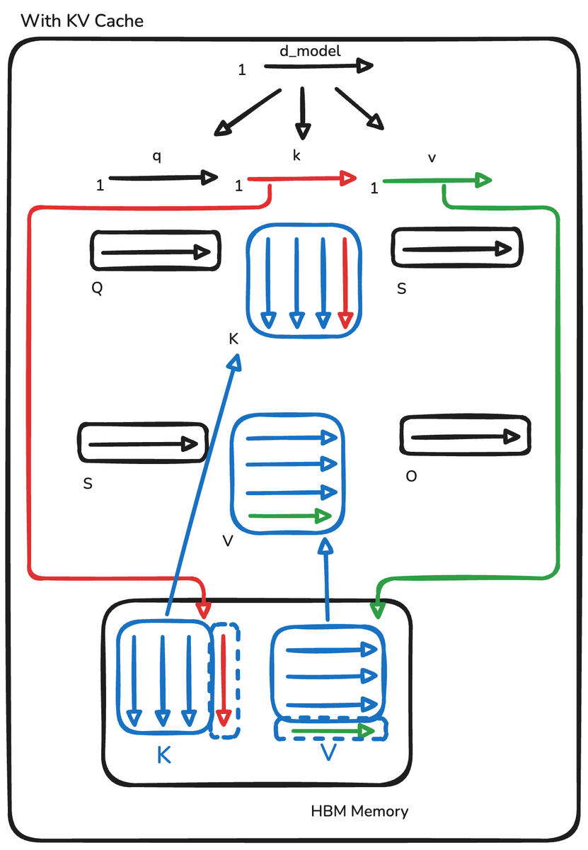
Notice the excessive reads and writes, which this paper replaces with:

def forward(self, x, mask=None, cache=None):
  # x is b,t,d
  b,t,d=x.shape
  d_head=d//self.num_heads
  h=self.num_heads
  qkv=self.qkv_proj(x)

  q=qkv[:, :, :d].view(b,t,h,d_head).transpose(1,2)
  k=qkv[:, :, d:2*d].view(b,t,h,d_head).transpose(1,2)
  v=qkv[:, :, 2*d:].view(b,t,h,d_head).transpose(1,2)
  
  k=F.elu(k)+1 
  k=k.transpose(-1,-2) 
  q=F.elu(q)+1
 
  S,z=cache if cache is not None else (0.0, 0.0)
  S=S+k@v
  z=z+k
      
 o=q@S #bhtd
 denom=q@z
 o_scaled=o/denom
 o_scaled=o_scaled.transpose(1,2).contiguous().view(b,t,d)
 o_proj=self.o_proj(o_scaled)
 cache=(S,z)
 
 return o_proj, cache

There is a trade-off.

Here, we replace the exponential used by softmax with ELU+1 applied separately to q and k before they interact. Both approaches normalize the resulting scores, but the feature map used by linear attention is a less expressive approximation of the softmax kernel. That approximation can reduce fidelity, although the practical accuracy loss depends on the architecture and workload.

Notice that we still divide by the sum of qk, which is omitted from the diagram for simplicity. At a high level, attention consists of three steps:

1. Make the qk scores non-negative. Linear attention uses ELU+1, while softmax uses exponentiation.
2. Divide by the sum.
3. Compute the weighted average of the values. This preserves the basic attention contract, but uses a less expressive feature map to make the QK scores non-negative.

def forward(self, x, mask=None, past_kv=None):
  # x is b,t,d
  b,t,d=x.shape
  d_head=d//self.num_heads
  h=self.num_heads
  qkv=self.qkv_proj(x)

  q=qkv[:, :, :d].view(b,t,h,d_head).transpose(1,2)
  k=qkv[:, :, d:2*d].view(b,t,h,d_head).transpose(1,2)
  v=qkv[:, :, 2*d:].view(b,t,h,d_head).transpose(1,2)

  # at prefill, q,k,v have shapes b,h,t,d
  # at decode, shape is b, h, 1, d
  # so i cat at the t dimension, dim(2)

  if past_kv is not None:
    k_past=past_kv[0]
    v_past=past_kv[1]
    k=torch.cat((k_past, k), dim=2)
    v=torch.cat((v_past, v), dim=2)

  scores=([email protected](-1,-2))/math.sqrt(d_head)
  if past_kv is None: #we're in prefill and need to mask
    causal_mask=torch.ones(t,t,dtype=bool, device=q.device)
    causal_mask=torch.triu(causal_mask, diagonal=1)
    scores=scores.masked_fill(causal_mask, float('-inf'))

  if mask is not None:
    scores=scores.masked_fill(~mask, float('-inf'))

  #get attn (bhtt x bhtd)
  attn=scores.softmax(-1)#bhtt
  o=attn@v #bhtd
  o=o.transpose(1,2).contiguous().view(b,t,d)  #b,t,d

  # use x to get qkv
  o_proj=self.o_proj(o)
  past_kv=(k, v)
  return o_proj, past_kv

def forward(self, x, mask=None, cache=None):
  # x is b,t,d
  b,t,d=x.shape
  d_head=d//self.num_heads
  h=self.num_heads
  qkv=self.qkv_proj(x)

  q=qkv[:, :, :d].view(b,t,h,d_head).transpose(1,2)
  k=qkv[:, :, d:2*d].view(b,t,h,d_head).transpose(1,2)
  v=qkv[:, :, 2*d:].view(b,t,h,d_head).transpose(1,2)
  
  k=F.elu(k)+1 
  k=k.transpose(-1,-2) 
  q=F.elu(q)+1
 
  S,z=cache if cache is not None else (0.0, 0.0)
  S=S+k@v
  z=z+k
      
 o=q@S #bhtd
 denom=q@z
 o_scaled=o/denom
 o_scaled=o_scaled.transpose(1,2).contiguous().view(b,t,d)
 o_proj=self.o_proj(o_scaled)
 cache=(S,z)
 
 return o_proj, cache

DeltaNet (Fast Weight Programmers)

A finite cache must overwrite or combine with information already stored. The state from token i-1 does not receive its own slot; it is added to the same D by D matrix. New queries can therefore no longer retrieve a perfectly isolated representation of each earlier token.

That addition is also the source of the efficiency gain. Updating the cache additively rather than by concatenation prevents it from growing in O(N), but the same operation causes information to interfere. DeltaNet addresses this loss of recoverability.

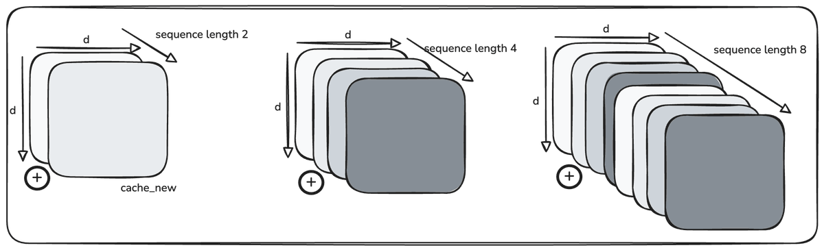
Eloquently put by Schlag’s paper (Fast Weight Programmers): “when the sequence length exceeds storage capacity, the model may end up in an overcapacity regime. To properly operate under such a regime, the model should learn to dynamically interact with the memory contents and selectively decide which key-value associations to keep and which ones to delete. The purely additive instruction may be inappropriate for this purpose…. endlessly adding new associations to a memory of finite size, as in Eq. 17, inevitably will reach a limit.“

The regime that makes linear attention attractive, where N is much larger than D, also exposes its main limitation. Once the state exceeds its effective capacity, associations begin to interfere because the update is additive and nothing leaves the cache.

def forward(self, x, mask=None, cache=None):
  # x is b,t,d
  b,t,d=x.shape
  d_head=d//self.num_heads
  h=self.num_heads
  qkv=self.qkv_proj(x)

  q=qkv[:, :, :d].view(b,t,h,d_head).transpose(1,2)
  k=qkv[:, :, d:2*d].view(b,t,h,d_head).transpose(1,2)
  v=qkv[:, :, 2*d:].view(b,t,h,d_head).transpose(1,2)

  q = F.normalize(F.silu(q), dim=-1)     
  k = F.normalize(F.silu(k), dim=-1)     
  beta = torch.sigmoid(self.w_beta(x)).view(b, 1, t, 1)   
  # new: per-token write strength

  S = cache if cache is not None else 0.0  

  v_old = k @ S # read the board at this key
  u = beta * (v - v_old) # the delta: only what's actually new
  S = S + k.transpose(-1, -2) @ u # same outer-product write as before

  o = q @ S # read, no denominator
  o = o.transpose(1, 2).contiguous().view(b, t, d)
  return self.o_proj(o), S

A visual example makes this easier to follow.

Take a single association written as S = k.T @ v. If read back with the same key and you get k @ (k.T @ v), which is (k @ k.T) v, which is the squared norm of k times v. So read returns scaled by key's squared norm, and if normalize k to unit length, or just divide result by norm, get v back exactly.

Q is also a learned pointer. Wq and Wk read the same residual stream, and the query for a fact points at the key direction that fact was written into. The update first asks what information the current key retrieves from the cache. It subtracts that existing information from the value we want to store, multiplies the key by the difference, and adds the result back. Old information is removed and new information is written in its place.

def forward(self, x, mask=None, cache=None):
  # x is b,t,d
  b,t,d=x.shape
  d_head=d//self.num_heads
  h=self.num_heads
  qkv=self.qkv_proj(x)

  q=qkv[:, :, :d].view(b,t,h,d_head).transpose(1,2)
  k=qkv[:, :, d:2*d].view(b,t,h,d_head).transpose(1,2)
  v=qkv[:, :, 2*d:].view(b,t,h,d_head).transpose(1,2)

  q = F.normalize(F.silu(q), dim=-1)     
  k = F.normalize(F.silu(k), dim=-1)     
  beta = torch.sigmoid(self.w_beta(x)).view(b, 1, t, 1)   
  # new: per-token write strength

  S = cache if cache is not None else 0.0  

  v_old = k @ S # read the board at this key
  u = beta * (v - v_old) # the delta: only what's actually new
  S = S + k.transpose(-1, -2) @ u # same outer-product write as before

  o = q @ S # read, no denominator
  o = o.transpose(1, 2).contiguous().view(b, t, d)
  return self.o_proj(o), S

DeltaNet (Parallelizing Linear Transformers with Delta Rule)

This is the most difficult section of the post. It took me about seven hours to develop a working understanding of it, so I will build the explanation from the implementation. In short, DeltaNet implements a first-order linear recurrence with generalized Householder transition matrices, enabling chunk-wise parallel forward passes for hardware-efficient linear-time training. It splits the inputs and outputs into several chunks of size C, and computes outputs for each chunk based on the final state of the previous chunk and the query key value blocks of the current chunk.

The practical problem is prefill. A direct implementation of the Delta rule over a sequence of T tokens would look like this:

S = torch.zeros(b, h, dh, dh) if cache is None else cache
outs = []
for i in range(t):
    k_i = k[:, :, i:i+1]  
    v_i = v[:, :, i:i+1]
    b_i = beta[:, :, i:i+1]
    v_old = k_i @ S                  
    u_i  = b_i * (v_i - v_old)
    S = S + k_i.transpose(-1, -2) @ u_i # write
    outs.append(q[:, :, i:i+1] @ S)     
o = torch.cat(outs, dim=2)                 

Unlike standard attention, this formulation requires a correction at every key vector, so the path to a parallel matrix multiplication is not immediately obvious. Even without the Delta rule, a direct linear-attention prefill remains sequential:

S = torch.zeros(b, h, dh, dh) if cache is None else cache
outs = []
for i in range(t):
    q = q[:, :, i:i+1]  
    k = k[:, :, i:i+1]  
    v = v[:, :, i:i+1]

    S=S_old+k@v
	  o=q@S #bhtd
	  o=self.norm(o)
    o=o.transpose(1, 2).contiguous().view(b, t, d)

    out=self.o_proj(o)
    cache=S
    outs.append(out)

o = torch.cat(outs, dim=2)

A chunked formulation provides a more efficient approach. The mechanics are easier to understand through an example:

Setting C=N recovers standard O(N^2) attention, while C=1 gives regular linear attention. Intermediate values we interpolate between trade additional within-chunk work for better hardware utilization. In practice, C is often 64 or 128 because tensor-core instructions operate efficiently at that granularity; UMMA is one example.

The intermediate tiles are folded into S as part of the state update:

S = torch.zeros(b, h, dh, dh) if cache is None else cache
outs = []
for i in range(t//C):
    q_c = q[:, :, i*C:(i+1)*C]  
    k_c = k[:, :, i*C:(i+1)*C]  
    v_c = v[:, :, i*C:(i+1)*C]

	  o_prev=q_c@S #this is everything up to this block
	  
	  attn=(q_c@k_c.transpose(-1,-2)).tril() #masked attention 
	  o_curr=attn@v_c
		  
		o=o_prev+o_curr
    
    S_new=k_c.transpose(-1,-2)@v_c #recurrent attention 
    S=S+S_new
    outs.append(o)

o = torch.cat(outs, dim=2)

Within a block, we do q(kᵀv). This is score first, the normal attention order with masking. Across blocks, we follow (kᵀv)q, so we’re doing recurrent order, state first. Attention grows in O(N²) and this does not. Inside a block I do real attention (the masked QKᵀ times V), and across blocks I fold everything into the state and read it back with one matmul. So the cost splits in two. There's a fixed piece, 2Ld², which is the state work and doesn't care about C at all. And there's a growing piece, 2LCd, which is the score matrices sitting on the diagonal. Full attention is just the case where C equals L, and then that second term becomes 2L²d, quadratic. So the smaller I make C, the fewer FLOPs I do.

C=1 is the cheapest option in pure FLOP terms, but not necessarily in wall-clock time. A GPU can complete more arithmetic faster when the work maps efficiently onto its matrix-multiply hardware.

The next step is to extend the same approach to DeltaNet.

The underlying issue is simple: the chunking method used for purely additive attention does not directly apply to the delta updates:

v_old = k_i @ S                  
u_i  = b_i * (v_i - v_old)

We need every single state in order to compute the information that needs to be subtracted out. We can't parallelize it the same way without some mathematical re-parameterization. The authors therefore rewrite the delta updates from:

u=v_new-v_old
S_t= S_(t-1)+K.T@u
o=q@S_T

Here, a sequential loop computes one delta per iteration. The reparameterized form is:

S_t = S_{t-1}(I − β_t k_t k_tᵀ)  +  β_t v_t k_tᵀ
o_t = S_t q_t

This formulation allows the chunked code to compute all C deltas at once:

def chunk_delta_rule_forward(Q, K, V, beta, C):
		# L: sequence length, d: head dimension
		L, d = Q.shape
		# chunking
		Q, K, V = map(lambda x: x.reshape(-1,C,d), [Q, K, V])
		beta = beta.reshape(-1, C)
		K_beta = K * beta.unsqueeze(-1)
		V_beta = V * beta.unsqueeze(-1)
		
		# compute eq. 10 with vectorized forward substitution for fast inverse
		T = -(K_beta @ K.t()).tril(-1)
		for i in range(1, C):
				T[i, :i] = T[i, :i] + (T[i, :, None] * T[:, :i]).sum(-2)
		
		T += torch.eye(C)
		W = T @ K_beta
		U = T @ V_beta

		# chunkwise parallel. Eq. 8-9
		S = torch.zeros(d, d)
		O = torch.empty_like(V)
		
		for i in range(L//C):
				q_i, k_i, w_i = Q[i], K[i], W[i]
				u_i = U[i] - w_i @ S # the corrections, all of one chunk
				o_inter = q_i @ S
				A_i = (q_i @ k_i.t()).tril() #qk.t
				o_intra = A_i @ u_i # attention @ v (with corrections, so u)
				S += k_i.t() @ u_i # update state with addition 
				O[i] = o_intra + o_inter #update output with flash + recurrent
		return O.reshape(L, d)

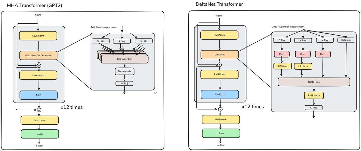
This gets us to our first comparison point: MHA vs DeltaNet Transformers:

S = torch.zeros(b, h, dh, dh) if cache is None else cache
outs = []
for i in range(t):
    k_i = k[:, :, i:i+1]  
    v_i = v[:, :, i:i+1]
    b_i = beta[:, :, i:i+1]
    v_old = k_i @ S                  
    u_i  = b_i * (v_i - v_old)
    S = S + k_i.transpose(-1, -2) @ u_i # write
    outs.append(q[:, :, i:i+1] @ S)     
o = torch.cat(outs, dim=2)                 

S = torch.zeros(b, h, dh, dh) if cache is None else cache
outs = []
for i in range(t):
    q = q[:, :, i:i+1]  
    k = k[:, :, i:i+1]  
    v = v[:, :, i:i+1]

    S=S_old+k@v
	  o=q@S #bhtd
	  o=self.norm(o)
    o=o.transpose(1, 2).contiguous().view(b, t, d)

    out=self.o_proj(o)
    cache=S
    outs.append(out)

o = torch.cat(outs, dim=2)

S = torch.zeros(b, h, dh, dh) if cache is None else cache
outs = []
for i in range(t//C):
    q_c = q[:, :, i*C:(i+1)*C]  
    k_c = k[:, :, i*C:(i+1)*C]  
    v_c = v[:, :, i*C:(i+1)*C]

	  o_prev=q_c@S #this is everything up to this block
	  
	  attn=(q_c@k_c.transpose(-1,-2)).tril() #masked attention 
	  o_curr=attn@v_c
		  
		o=o_prev+o_curr
    
    S_new=k_c.transpose(-1,-2)@v_c #recurrent attention 
    S=S+S_new
    outs.append(o)

o = torch.cat(outs, dim=2)

v_old = k_i @ S                  
u_i  = b_i * (v_i - v_old)

u=v_new-v_old
S_t= S_(t-1)+K.T@u
o=q@S_T

S_t = S_{t-1}(I − β_t k_t k_tᵀ)  +  β_t v_t k_tᵀ
o_t = S_t q_t

def chunk_delta_rule_forward(Q, K, V, beta, C):
		# L: sequence length, d: head dimension
		L, d = Q.shape
		# chunking
		Q, K, V = map(lambda x: x.reshape(-1,C,d), [Q, K, V])
		beta = beta.reshape(-1, C)
		K_beta = K * beta.unsqueeze(-1)
		V_beta = V * beta.unsqueeze(-1)
		
		# compute eq. 10 with vectorized forward substitution for fast inverse
		T = -(K_beta @ K.t()).tril(-1)
		for i in range(1, C):
				T[i, :i] = T[i, :i] + (T[i, :, None] * T[:, :i]).sum(-2)
		
		T += torch.eye(C)
		W = T @ K_beta
		U = T @ V_beta

		# chunkwise parallel. Eq. 8-9
		S = torch.zeros(d, d)
		O = torch.empty_like(V)
		
		for i in range(L//C):
				q_i, k_i, w_i = Q[i], K[i], W[i]
				u_i = U[i] - w_i @ S # the corrections, all of one chunk
				o_inter = q_i @ S
				A_i = (q_i @ k_i.t()).tril() #qk.t
				o_intra = A_i @ u_i # attention @ v (with corrections, so u)
				S += k_i.t() @ u_i # update state with addition 
				O[i] = o_intra + o_inter #update output with flash + recurrent
		return O.reshape(L, d)

Gated Delta Net

We now have a method for making precise changes to the cache. With each new fact (each new key vector), we can look at exactly the old information stored at that point and replace it with the new information we want to attend to.

However, this mechanism can forget only an association for which it has a specific replacement. It cannot efficiently clear multiple associations during a context switch or decay memory generally to free capacity.

If we were doing purely additive linear attention:

Adding the ability to forget would be simple. We'd just need a parameter controlling the forgetful state:

S_old=cache
S_new=k@v
# cache=S_old+S_new
cache=alpha * S_old + S_new

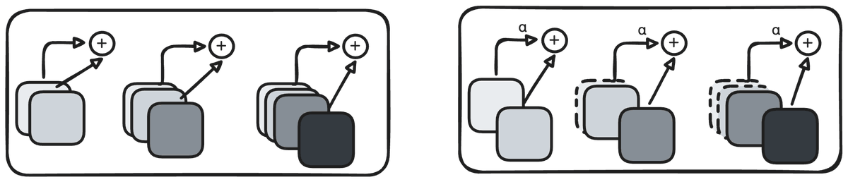
This is the Mamba-2 contribution. We decay the previous cache, then add the new cache at full strength, preventing the state from growing without bound.

Uniformly decaying all key-value associations at each time step by a dynamic ratio is a working approach, and it's what Mamba does. But it doesn't account for the varying importance of different key-value associations.

That is, if the model needs to forget one specific association, all associations are forgotten equally. The Delta rule, in contrast, can update a single fact but has no way to make the rest of the facts decay.

So the Gated Delta rule combines Mamba's gated update rule with the Delta rule. It adds a parameter, alpha, that switches to the pure Delta rule when set to one and clears the memory when set to zero. The challenge is implementing this with the same parallel-chunks method.

The implementation uses the same DeltaNet reparameterization described in the previous section. The mathematics is nearly identical, with one addition: a data-dependent scalar between zero and one that controls the decay of the previous state. This combines effective key-value association learning with adaptive memory management.

The corresponding code changes are shown below:

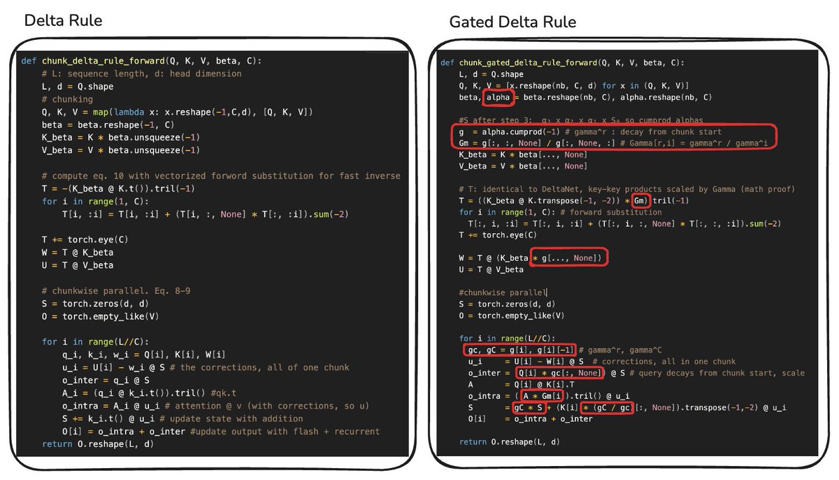
The γʳ/γⁱ term accounts for cumulative decay. A token written at time step x and read at x+t has been multiplied by αₓαₓ₊₁αₓ₊₂…αₓ₊ₜ. This is the multiplicative analogue of a prefix-sum calculation.

The resulting architecture looks like this:

S_old=cache
S_new=k@v
# cache=S_old+S_new
cache=alpha * S_old + S_new

KDA/Kimi Linear

At this point, researchers began experimenting with hybrid models that combine multiple forms of attention within one architecture, like Gated DeltaNet withM Mamba.

Kimi Linear drew attention for one central claim: under controlled comparisons, it outperformed full attention. The authors presented it as a drop-in architectural replacement with better quality and up to 6x higher decode throughput.

Kimi Linear improves on Gated DeltaNet by introducing fine-grained gating. Instead of a single scalar decay, it learns a separate decay value for each channel.

The KDA update rule remains similar, but the code now looks more like this:

Here, alpha.reshape(nb, C, d) captures the paper’s most significant contribution: fine-grained control over memory decay.

Placed beside the DeltaNet Transformer, the Kimi Linear architecture introduces three major changes:

1. It uses a hybrid system that interleaves Multi-head Latent Attention (MLA) layers.
2. It replaces the MLP with a Mixture-of-Experts (MoE) layer.
3. It adds capacity to DeltaNet through the alpha projection.

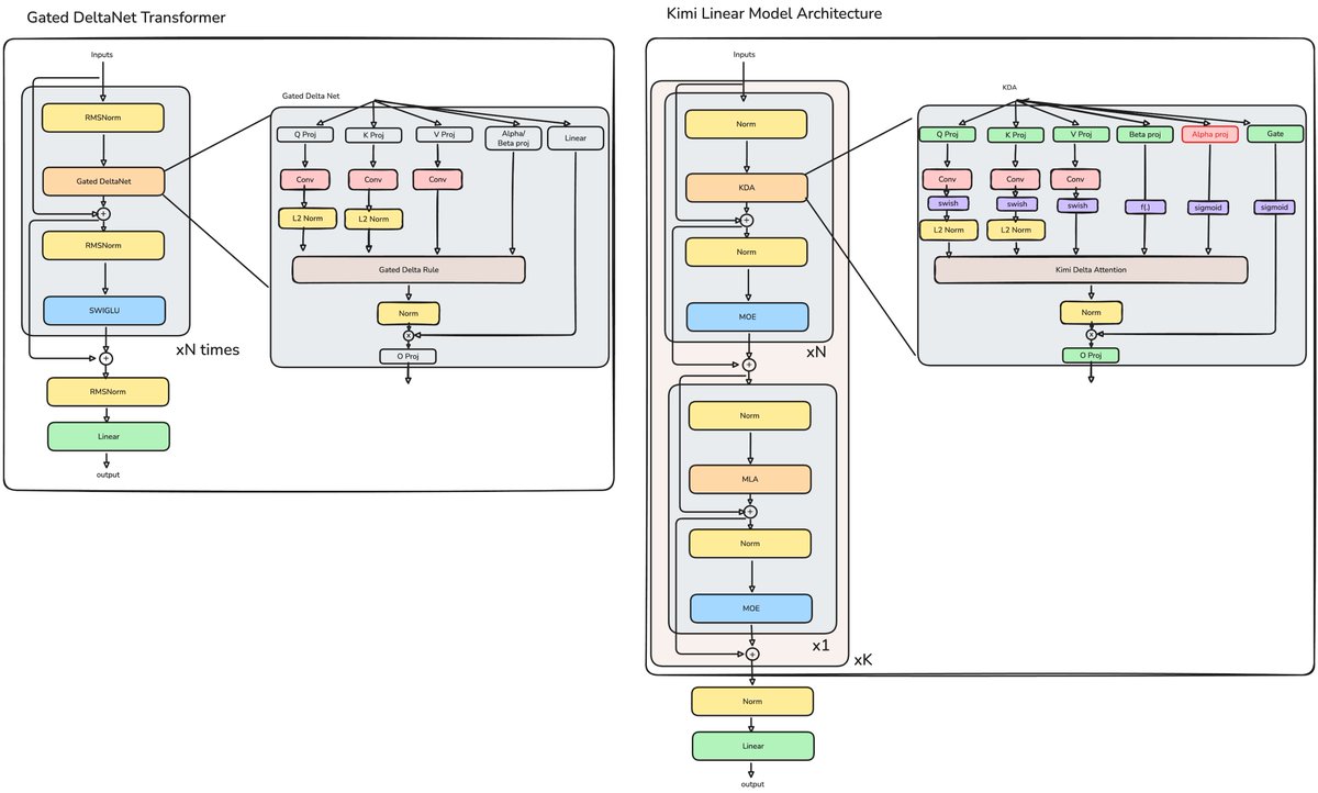
The later sections cover MLA and MoE in more detail. For now, the important point is that this is not blind scaling. The additional capacity has a specific mathematical purpose: the per-channel scale gives the model finer control over memory decay.

Scaling laws remain relevant, but capacity must be added in the right place and in a form the system can use. Each architecture in this progression adds capacity to address a concrete limitation in the preceding system.

Kimi K3

Ultimately, the KimiK3 language backbone looks similar to the Kimi Linear model above. It contains 23 four-layer macrocycles. In each macrocycle, three layers use Kimi Delta Attention and the fourth uses Multi-head Latent Attention. The first layer uses a dense feed-forward network; every remaining layer uses a latent Mixture-of-Experts.

At first glance, the changes from Kimi Linear appear modest:

• A substantial increase in scale
• Blockwise AttnRes every 12 layers
• MLA query LoRA and output gating
• Latent-space MoE
• SiTU activations
• Gated MLA KDA supplies constant-state recurrent memory, while periodic MLA layers retain full softmax retrieval over the context. The following simplified visualization provides a useful reference for the changes discussed below.

We will begin with the more direct changes: Gated MLA, latent-space MoE, and SiTU activations.

Gated MLA determines how much of each retrieved feature passes from MLA into the residual stream. It does this through element-wise multiplication with a gate projected from the input.

In a conventional MoE, a learned router uses dot-product similarity to send each token to a subset of expert networks. KimiK3 has 898 experts in total. Two are shared and process every token; of the remaining 896, the router selects 16 for each token.

KimiK3 also changes the expert activation. Instead of applying SiLU to the up projection, multiplying it element-wise by the gate, and then applying the down projection, it uses SiTU:

d = x.shape[-1] // 2
gate = x[..., :d].to(torch.float32)
up = x[..., d:].to(torch.float32)
situ_a = self.beta * torch.tanh(gate / self.beta) * torch.sigmoid(gate)
if self.linear_beta is not None:
    up = self.linear_beta * torch.tanh(up / self.linear_beta)
return (situ_a * up).to(x.dtype)

The model also down-projects inputs to the shared experts and up-projects their final sum:

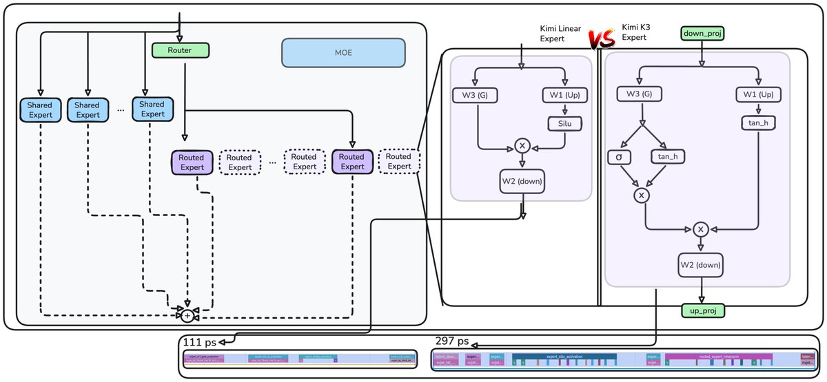
This illustrates a recurring challenge in model inference. Without a fused kernel, the new activation is almost 3x slower than the original path. One offsetting optimization is that the experts operate in a compressed latent space, which makes their forward pass much faster and nearly halves the FLOPs.

The remaining changes are MLA query LoRA, output gating, and blockwise Attention Residuals every 12 layers. AttnRes adds roughly 2% inference latency, but provides two important benefits:

• Selective retrieval of earlier representations, which mitigates residual dilution and hidden-state growth
• A 1.25x compute advantage AttnRes and MLA address the same underlying limitation from different directions. KDA layers operate with constant-size state and must inevitably discard information. MLA retrieves from the token context, while AttnRes retrieves from earlier depth-wise representations.

d = x.shape[-1] // 2
gate = x[..., :d].to(torch.float32)
up = x[..., d:].to(torch.float32)
situ_a = self.beta * torch.tanh(gate / self.beta) * torch.sigmoid(gate)
if self.linear_beta is not None:
    up = self.linear_beta * torch.tanh(up / self.linear_beta)
return (situ_a * up).to(x.dtype)

AttnRes

Thanks to @chloey3k for help with this section. In each forward pass, the input passes through a stack of layers. Here, each layer consists of an attention block (KDA or MLA) and an MLP or MoE block. Normally, the input to each layer is the sum of the original embedding and every preceding layer's output, all weighted equally.

Here, h_i is the input to layer i, h_1 is the embedding of the current token (the last token in the sequence so far), and f_i(h_i) is the output of layer i (an attention or MLP block).

The problem is the lack of selective access. Different layer types receive the same aggregated state, even though they may benefit from different weightings. Because the recurrence is purely additive, later layers must also learn increasingly large outputs to influence the accumulated residual, which can destabilize training. Instead of treating all the layers equally, AttnRes multiplies each term of that sum by a specialized weight, which lets the model give more importance to whichever layers are most useful in context.

Each weight alpha_i is computed from a query-key dot product. The query is learned for each layer, while the keys and values come from earlier residual-stream states. The scores are normalized to sum to one, then used to form a weighted combination of those states.

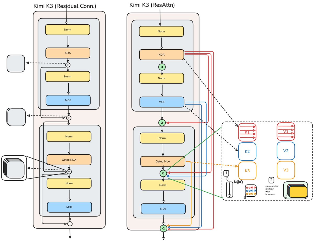
The model therefore does not have to condition only on its immediate predecessor. AttnRes gives each layer selective access to earlier layer outputs, allowing its learned query to retrieve the representations most useful for the current computation.

The pseudocode below applies the same idea at block granularity. A block is the element-wise sum of the attention and MLP outputs accumulated across 12 decoder layers, stored as a single depth representation for later AttnRes mixing.

Applying residual attention at every layer would add too much training and inference cost. Applying it only at fixed block boundaries captures most of the benefit at a lower cost. In KimiK3, each boundary occurs after 12 decoder layers. Across 23 four-layer macrocycles, this produces eight AttnRes blocks, which increases our inference speed.

This is possibly the most important part of the block_attn_res function

V = torch.stack(blocks + [partial_block]) # [N+1, B, T, D]
K = norm(V)
logits = torch.einsum('d, n b t d -> n b t', proj.weight.squeeze(), K)
h = torch.einsum('n b t, n b t d -> b t d', logits.softmax(0), V)
return h

This completes the progression from GPT-2 to KimiK3.

The central change is not scale alone. Each architectural step changes what the model stores, how it updates that state, or how it retrieves information that a fixed-size state cannot preserve.

KimiK3 combines constant-state recurrent memory, periodic softmax retrieval, sparse expert capacity, and selective depth-wise residual access. The result is a system that spends additional capacity where it has a specific functional role.

In essence, a fixed-capacity associative memory (fixed dimensions) needs an eviction policy, since a purely additive linear operation eventually adds interference once at capacity. To that end, learned selection, like gating, routing, or decay, is necessary, and attention is the most effective selective-read mechanism.

V = torch.stack(blocks + [partial_block]) # [N+1, B, T, D]
K = norm(V)
logits = torch.einsum('d, n b t d -> n b t', proj.weight.squeeze(), K)
h = torch.einsum('n b t, n b t d -> b t d', logits.softmax(0), V)
return h